Introduction to combinatorics in Sage#

This thematic tutorial is a translation by Hugh Thomas of the combinatorics chapter written by Nicolas M. Thiéry in the book “Calcul Mathématique avec Sage” [CMS2012]. It covers mainly the treatment in Sage of the following combinatorial problems: enumeration (how many elements are there in a set \(S\)?), listing (generate all the elements of \(S\), or iterate through them), and random selection (choosing an element at random from a set \(S\) according to a given distribution, for example the uniform distribution). These questions arise naturally in the calculation of probabilities (what is the probability in poker of obtaining a straight or a four-of-a-kind of aces?), in statistical physics, and also in computer algebra (the number of elements in a finite field), or in the analysis of algorithms. Combinatorics covers a much wider domain (partial orders, representation theory, …) for which we only give a few pointers towards the possibilities offered by Sage.

Todo

Add link to some thematic tutorial on graphs

A characteristic of computational combinatorics is the profusion of types of objects and sets that one wants to manipulate. It would be impossible to describe them all or, a fortiori, to implement them all. After some Initial examples, this chapter illustrates the underlying method: supplying the basic building blocks to describe common combinatorial sets Common enumerated sets, tools for combining them to construct new examples Constructions, and generic algorithms for solving uniformly a large class of problems Generic algorithms.

This is a domain in which Sage has much more extensive capabilities than most computer algebra systems, and it is rapidly expanding; at the same time, it is still quite new, and has many unnecessary limitations and incoherences.

Initial examples#

Poker and probability#

We begin by solving a classic problem: enumerating certain combinations of cards in the game of poker, in order to deduce their probability.

A card in a poker deck is characterized by a suit (hearts, diamonds, spades, or clubs) and a value (2, 3, …, 10, jack, queen, king, ace). The game is played with a full deck, which consists of the Cartesian product of the set of suits and the set of values:

\[\operatorname{Cards} = \operatorname{Suits} \times \operatorname{Values} = \{ (s, v) \mathrel| s\in \operatorname{Suits} \text{ et } v \in \operatorname{Values} \}\,.\]

We construct these examples in Sage:

sage: Suits = Set(["Hearts", "Diamonds", "Spades", "Clubs"])
sage: Values = Set([2, 3, 4, 5, 6, 7, 8, 9, 10,
....:               "Jack", "Queen", "King", "Ace"])
sage: Cards = cartesian_product([Values, Suits])

There are \(4\) suits and \(13\) possible values, and therefore \(4\times 13=52\) cards in the poker deck:

sage: Suits.cardinality()
4
sage: Values.cardinality()
13
sage: Cards.cardinality()
52

Draw a card at random:

sage: Cards.random_element()                      # random
(6, 'Clubs')

Now we can define a set of cards:

sage: Set([Cards.random_element(), Cards.random_element()])  # random
{(2, 'Hearts'), (4, 'Spades')}

This problem should eventually disappear: it is planned to change the implementation of Cartesian products so that their elements are immutable by default.

Returning to our main topic, we will be considering a simplified version of poker, in which each player directly draws five cards, which form his hand. The cards are all distinct and the order in which they are drawn is irrelevant; a hand is therefore a subset of size \(5\) of the set of cards. To draw a hand at random, we first construct the set of all possible hands, and then we ask for a randomly chosen element:

sage: Hands = Subsets(Cards, 5)
sage: Hands.random_element()                      # random
{(4, 'Hearts', 4), (9, 'Diamonds'), (8, 'Spades'),
 (9, 'Clubs'), (7, 'Hearts')}

The total number of hands is given by the number of subsets of size \(5\) of a set of size \(52\), which is given by the binomial coefficient \(\binom{52}{5}\):

sage: binomial(52,5)
2598960

One can also ignore the method of calculation, and simply ask for the size of the set of hands:

sage: Hands.cardinality()
2598960

The strength of a poker hand depends on the particular combination of cards present. One such combination is the flush; this is a hand all of whose cards have the same suit. (In principle, straight flushes should be excluded; this will be the goal of an exercise given below.) Such a hand is therefore characterized by the choice of five values from among the thirteen possibilities, and the choice of one of four suits. We will construct the set of all flushes, so as to determine how many there are:

sage: Flushes = cartesian_product([Subsets(Values, 5), Suits])
sage: Flushes.cardinality()
5148

The probability of obtaining a flush when drawing a hand at random is therefore:

sage: Flushes.cardinality()  / Hands.cardinality()
33/16660

or about two in a thousand:

sage: 1000.0 * Flushes.cardinality()  / Hands.cardinality()
1.98079231692677

We will now attempt a little numerical simulation. The following function tests whether a given hand is a flush or not:

sage: def is_flush(hand):
....:     return len(set(suit for (val, suit) in hand)) == 1

We now draw 10000 hands at random, and count the number of flushes obtained (this takes about 10 seconds):

sage: n = 10000
sage: nflush = 0
sage: for i in range(n):                            # long time
....:    hand = Hands.random_element()
....:    if is_flush(hand):
....:        nflush += 1
sage: n, nflush                               # random
(10000, 18)

Exercises

A hand containing four cards of the same value is called a four of a kind. Construct the set of four of a kind hands (Hint: use Arrangements to choose a pair of distinct values at random, then choose a suit for the first value). Calculate the number of four of a kind hand, list them, and then determine the probability of obtaining a four of a kind when drawing a hand at random.

A hand all of whose cards have the same suit, and whose values are consecutive, is called a straight flush rather than a flush. Count the number of straight flushes, and then deduce the correct probability of obtaining a flush when drawing a hand at random.

Calculate the probability of each of the poker hands (see Wikipedia article Poker_hands), and compare them with the results of simulations.

Enumeration of trees using generating functions#

In this section, we discuss the example of complete binary trees, and illustrate in this context many techniques of enumeration in which formal power series play a natural role. These techniques are quite general, and can be applied whenever the combinatorial objects in question admit a recursive definition (grammar) (see Species, decomposable combinatorial classes for an automated treatment). The goal is not a formal presentation of these methods; the calculations are rigorous, but most of the justifications will be skipped.

A complete binary tree is either a leaf \(\mathrm{L}\), or a node to which two complete binary trees are attached (see Figure: The five complete binary trees with four leaves).

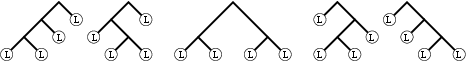
../../_images/complete-binary-trees-4.png — Figure: The five complete binary trees with four leaves#

Exercise: enumeration of binary trees

Find by hand all the complete binary trees with \(n=1, 2, 3, 4, 5\) leaves (see Exercise: complete binary tree iterator to find them using Sage).

Our goal is to determine the number \(c_n\) of complete binary trees with \(n\) leaves (in this section, except when explicitly stated otherwise, “trees” always means complete binary trees). This is a typical situation in which one is not only interested in a single set, but in a family of sets, typically parameterized by \(n\in \NN\).

According to the solution of Exercise: enumeration of binary trees, the first terms are given by \(c_1,\dots,c_5=1,1,2,5,14\). The simple fact of knowing these few numbers is already very valuable. In fact, this permits research in a gold mine of information: the Online Encyclopedia of Integer Sequences, commonly called “Sloane”, the name of its principal author, which contains more than 190000 sequences of integers:

sage: oeis([1,1,2,5,14])                            # optional -- internet
A000108: Catalan numbers: ...
...
...

The result suggests that the trees are counted by one of the most famous sequences, the Catalan numbers. Looking through the references supplied by the Encyclopedia, we see that this is really the case: the few numbers above form a digital fingerprint of our objects, which enable us to find, in a few seconds, a precise result from within an abundant literature.

Our next goal is to recover this result using Sage. Let \(C_n\) be the set of trees with \(n\) leaves, so that \(c_n=|C_n|\); by convention, we will define \(C_0=\emptyset\) and \(c_0=0\). The set of all trees is then the disjoint union of the sets \(C_n\):

\[C=\biguplus_{n\in \mathbb N} C_n\,.\]

Having named the set \(C\) of all trees, we can translate the recursive definition of trees into a set-theoretic equation:

\[C \quad \approx \quad \{ \mathrm{L} \} \quad \uplus\quad C \times C\,.\]

In words: a tree \(t\) (which is by definition in \(C\)) is either a leaf (so in \(\{\mathrm{L}\}\)) or a node to which two trees \(t_1\) and \(t_2\) have been attached, and which we can therefore identify with the pair \((t_1,t_2)\) (in the Cartesian product \(C\times C\)).

The founding idea of algebraic combinatorics, introduced by Euler in a letter to Goldbach of 1751 to treat a similar problem , is to manipulate all the numbers \(c_n\) simultaneously, by encoding them as coefficients in a formal power series, called the generating function of the \(c_n\)’s:

\[C(z) = \sum_{n\in \mathbb N} c_n z^n\,,\]

where \(z\) is a formal variable (which means that we do not have to worry about questions of convergence). The beauty of this idea is that set-theoretic operations \((A\uplus B\), \(A\times B)\) translate naturally into algebraic operations on the corresponding series (\(A(z)+B(z)\), \(A(z)\cdot B(z)\)), in such a way that the set-theoretic equation satisfied by \(C\) can be translated directly into an algebraic equation satisfied by \(C(z)\):

\[C(z) = z + C(z) \cdot C(z)\,.\]

Now we can solve this equation with Sage. In order to do so, we introduce two variables, \(C\) and \(z\), and we define the equation:

sage: C, z = var('C,z')
sage: sys = [ C == z + C*C ]

There are two solutions, which happen to have closed forms:

sage: sol = solve(sys, C, solution_dict=True); sol
[{C: -1/2*sqrt(-4*z + 1) + 1/2}, {C: 1/2*sqrt(-4*z + 1) + 1/2}]
sage: s0 = sol[0][C]; s1 = sol[1][C]

and whose Taylor series begin as follows:

sage: s0.series(z, 6)
1*z + 1*z^2 + 2*z^3 + 5*z^4 + 14*z^5 + Order(z^6)
sage: s1.series(z, 6)
1 + (-1)*z + (-1)*z^2 + (-2)*z^3 + (-5)*z^4 + (-14)*z^5
+ Order(z^6)

The second solution is clearly aberrant, while the first one gives the expected coefficients. Therefore, we set:

sage: C = s0

We can now calculate the next terms:

sage: C.series(z, 11)
1*z + 1*z^2 + 2*z^3 + 5*z^4 + 14*z^5 + 42*z^6 +
132*z^7 + 429*z^8 + 1430*z^9 + 4862*z^10 + Order(z^11)

or calculate, more or less instantaneously, the 100-th coefficient:

sage: C.series(z, 101).coefficient(z,100)
227508830794229349661819540395688853956041682601541047340

It is unfortunate to have to recalculate everything if at some point we wanted the 101-st coefficient. Lazy power series (see sage.rings.lazy_series_ring) come into their own here, in that one can define them from a system of equations without solving it, and, in particular, without needing a closed form for the answer. We begin by defining the ring of lazy power series:

sage: L.<z> = LazyPowerSeriesRing(QQ)

Then we create a “free” power series, which we name, and which we then define by a recursive equation:

sage: C = L.undefined(valuation=1)
sage: C.define( z + C * C )

sage: [C.coefficient(i) for i in range(11)]
[0, 1, 1, 2, 5, 14, 42, 132, 429, 1430, 4862]

At any point, one can ask for any coefficient without having to redefine \(C\):

sage: C.coefficient(100)
227508830794229349661819540395688853956041682601541047340
sage: C.coefficient(200)
129013158064429114001222907669676675134349530552728882499810851598901419013348319045534580850847735528275750122188940

We now return to the closed form of \(C(z)\):

sage: z = var('z')
sage: C = s0; C
-1/2*sqrt(-4*z + 1) + 1/2

The \(n\)-th coefficient in the Taylor series for \(C(z)\) being given by \(\frac{1}{n!} C(z)^{(n)}(0)\), we look at the successive derivatives \(C(z)^{(n)}(z)\):

sage: derivative(C, z, 1)
1/sqrt(-4*z + 1)
sage: derivative(C, z, 2)
2/(-4*z + 1)^(3/2)
sage: derivative(C, z, 3)
12/(-4*z + 1)^(5/2)

This suggests the existence of a simple explicit formula, which we will now seek. The following small function returns \(d_n=n! \, c_n\):

sage: def d(n): return derivative(s0, n).subs(z=0)

Taking successive quotients:

sage: [ (d(n+1) / d(n)) for n in range(1,17) ]
[2, 6, 10, 14, 18, 22, 26, 30, 34, 38, 42, 46, 50, 54, 58, 62]

we observe that \(d_n\) satisfies the recurrence relation \(d_{n+1}=(4n-2)d_n\), from which we deduce that \(c_n\) satisfies the recurrence relation \(c_{n+1}=\frac{(4n-2)}{n+1}c_n\). Simplifying, we find that \(c_n\) is the \((n-1)\)-th Catalan number:

\[c_n = \operatorname{Catalan}(n-1) = \frac {1}{n} \binom{2(n-1)}{n-1}\,.\]

We check this:

sage: n = var('n')
sage: c = 1/n*binomial(2*(n-1),n-1)
sage: [c.subs(n=k) for k in range(1, 11)]
[1, 1, 2, 5, 14, 42, 132, 429, 1430, 4862]
sage: [catalan_number(k-1) for k in range(1, 11)]
[1, 1, 2, 5, 14, 42, 132, 429, 1430, 4862]

We can now calculate coefficients much further; here we calculate \(c_{100000}\) which has more than \(60000\) digits:

sage: cc = c(n = 100000)

This takes a couple of seconds:

sage: %time cc = c(100000)                         # not tested
CPU times: user 2.34 s, sys: 0.00 s, total: 2.34 s
Wall time: 2.34 s
sage: ZZ(cc).ndigits()
60198

The methods which we have used generalize to all recursively defined objects: the system of set-theoretic equations can be translated into a system of equations on the generating function, which enables the recursive calculation of its coefficients. If the set-theoretic equations are simple enough (for example, if they only involve Cartesian products and disjoint unions), the equation for \(C(z)\) is algebraic. This equation has, in general, no closed-form solution. However, using confinement, one can deduce a linear differential equation which \(C(z)\) satisfies. This differential equation, in turn, can be translated into a recurrence relation of fixed length on its coefficients \(c_n\). In this case, the series is called D-finite. After the initial calculation of this recurrence relation, the calculation of coefficients is very fast. All these steps are purely algorithmic, and it is planned to port into Sage the implementations which exist in Maple (the gfun and combstruct packages) or MuPAD-Combinat (the decomposableObjects library).

For the moment, we illustrate this general procedure in the case of complete binary trees. The generating function \(C(z)\) is a solution to an algebraic equation \(P(z,C(z)) = 0\), where \(P=P(x,y)\) is a polynomial with coefficients in \(\QQ\). In the present case, \(P=y^2-y+x\). We formally differentiate this equation with respect to \(z\):

sage: x, y, z = var('x, y, z')
sage: P = function('P')(x, y)
sage: C = function('C')(z)
sage: equation =  P(x=z, y=C) == 0
sage: diff(equation, z)
diff(C(z), z)*D[1](P)(z, C(z)) + D[0](P)(z, C(z)) == 0

or, in a more readable format,

\[\frac{d C(z)}{d z} \frac{\partial P}{\partial y} (z, C(z)) + \frac{\partial P}{\partial x}(z,C(z)) = 0\]

From this we deduce:

\[\frac{d C(z)}{d z} = - \frac{\frac{\partial P}{\partial x}}{\frac{\partial P}{\partial y}}(z, C(z))\,.\]

In the case of complete binary trees, this gives:

sage: P = y^2 - y + x
sage: Px = diff(P, x); Py = diff(P, y)
sage: - Px / Py
-1/(2*y - 1)

Recall that \(P(z, C(z))=0\). Thus, we can calculate this fraction mod \(P\) and, in this way, express the derivative of \(C(z)\) as a polynomial in \(C(z)\) with coefficients in \(\QQ(z)\). In order to achieve this, we construct the quotient ring \(R= \QQ(x)[y]/ (P)\):

sage: Qx = QQ['x'].fraction_field()
sage: Qxy = Qx['y']
sage: R = Qxy.quo(P); R
Univariate Quotient Polynomial Ring in ybar
over Fraction Field of Univariate Polynomial Ring in x
over Rational Field with modulus y^2 - y + x

Note: ybar is the name of the variable \(y\) in the quotient ring.

Todo

add link to some tutorial on quotient rings

We continue the calculation of this fraction in \(R\):

sage: fraction = - R(Px) / R(Py); fraction
(1/2/(x - 1/4))*ybar - 1/4/(x - 1/4)

Note

The following variant does not work yet:

sage: fraction = R( - Px / Py ); fraction   # todo: not implemented
Traceback (most recent call last):
...
TypeError: denominator must be a unit

We lift the result to \(\QQ(x)[y]\) and then substitute \(z\) and \(C(z)\) to obtain an expression for \(\frac{d}{dz}C(z)\):

sage: fraction = fraction.lift(); fraction
(1/2/(x - 1/4))*y - 1/4/(x - 1/4)
sage: fraction(x=z, y=C)
2*C(z)/(4*z - 1) - 1/(4*z - 1)

or, more legibly,

\[\frac{\partial C(z)}{\partial z} = \frac{1}{1-4z} -\frac{2}{1-4z}C(z)\,.\]

In this simple case, we can directly deduce from this expression a linear differential equation with coefficients in \(\QQ[z]\):

sage: equadiff = diff(C,z) == fraction(x=z, y=C)
sage: equadiff
diff(C(z), z) == 2*C(z)/(4*z - 1) - 1/(4*z - 1)
sage: equadiff = equadiff.simplify_rational()
sage: equadiff = equadiff * equadiff.rhs().denominator()
sage: equadiff = equadiff - equadiff.rhs()
sage: equadiff
(4*z - 1)*diff(C(z), z) - 2*C(z) + 1 == 0

or, more legibly,

\[(1-4z) \frac{\partial C(z)}{\partial z} + 2 C(z) - 1 = 0\,.\]

It is trivial to verify this equation on the closed form:

sage: Cf = sage.symbolic.function_factory.function('C')
sage: equadiff.substitute_function(Cf, s0.function(z))
(4*z - 1)/sqrt(-4*z + 1) + sqrt(-4*z + 1) == 0
sage: bool(equadiff.substitute_function(Cf, s0.function(z)))
True

In the general case, one continues to calculate successive derivatives of \(C(z)\). These derivatives are confined in the quotient ring \(\QQ(z)[C]/(P)\) which is of finite dimension \(\deg P\) over \(\QQ(z)\). Therefore, one will eventually find a linear relation among the first \(\deg P\) derivatives of \(C(z)\). Putting it over a single denominator, we obtain a linear differential equation of degree \(\leq \deg P\) with coefficients in \(\QQ[z]\). By extracting the coefficient of \(z^n\) in the differential equation, we obtain the desired recurrence relation on the coefficients; in this case we recover the relation we had already found, based on the closed form:

\[c_{n+1}=\frac{(4n-2)}{n+1}c_n\]

After fixing the correct initial conditions, it becomes possible to calculate the coefficients of \(C(z)\) recursively:

sage: def C(n): return 1 if n <= 1 else (4*n-6)/n * C(n-1)
sage: [ C(i) for i in range(10) ]
[1, 1, 1, 2, 5, 14, 42, 132, 429, 1430]

If \(n\) is too large for the explicit calculation of \(c_n\), a sequence asymptotically equivalent to the sequence of coefficients \(c_n\) may be sought. Here again, there are generic techniques. The central tool is complex analysis, specifically, the study of the generating function around its singularities. In the present instance, the singularity is at \(z_0=1/4\) and one would obtain \(c_n \sim \frac{4^n}{n^{3/2}\sqrt{\pi}}\).

Summary#

We see here a general phenomenon of computer algebra: the best data structure to describe a complicated mathematical object (a real number, a sequence, a formal power series, a function, a set) is often an equation defining the object (or a system of equations, typically with some initial conditions). Attempting to find a closed-form solution to this equation is not necessarily of interest: on the one hand, such a closed form rarely exists (e.g., the problem of solving a polynomial by radicals), and on the other hand, the equation, in itself, contains all the necessary information to calculate algorithmically the properties of the object under consideration (e.g., a numerical approximation, the initial terms or elements, an asymptotic equivalent), or to calculate with the object itself (e.g., performing arithmetic on power series). Therefore, instead of solving the equation, we look for the equation describing the object which is best suited to the problem we want to solve.

As we saw in our example, confinement (for example, in a finite dimensional vector space) is a fundamental tool for studying such equations. This notion of confinement is widely applicable in elimination techniques (linear algebra, Gröbner bases, and their algebro-differential generalizations). The same tool is central in algorithms for automatic summation and automatic verification of identities (Gosper’s algorithm, Zeilberger’s algorithm, and their generalizations; see also Exercise: alternating sign matrices).

Todo

add link to some tutorial on summation

All these techniques and their many generalizations are at the heart of very active topics of research: automatic combinatorics and analytic combinatorics, with major applications in the analysis of algorithms. It is likely, and desirable, that they will be progressively implemented in Sage.

Common enumerated sets#

First example: the subsets of a set#

Fix a set \(E\) of size \(n\) and consider the subsets of \(E\) of size \(k\). We know that these subsets are counted by the binomial coefficients \(\binom n k\). We can therefore calculate the number of subsets of size \(k=2\) of \(E=\{1,2,3,4\}\) with the function binomial:

sage: binomial(4, 2)
6

Alternatively, we can construct the set \(\mathcal P_2(E)\) of all the subsets of size \(2\) of \(E\), then ask its cardinality:

sage: S = Subsets([1,2,3,4], 2)
sage: S.cardinality()
6

Once S has been constructed, we can also obtain the list of its elements:

sage: S.list()
[{1, 2}, {1, 3}, {1, 4}, {2, 3}, {2, 4}, {3, 4}]

or select an element at random:

sage: S.random_element()                 # random
{1, 4}

More precisely, the object S models the set \(\mathcal P_2(E)\) equipped with a fixed order (here, lexicographic order). It is therefore possible to ask for its \(5\)-th element, keeping in mind that, as with Python lists, the first element is numbered zero:

sage: S.unrank(4)
{2, 4}

As a shortcut, in this setting, one can also use the notation:

sage: S[4]
{2, 4}

but this should be used with care because some sets have a natural indexing other than by \((0, 1, \dots)\).

Conversely, one can calculate the position of an object in this order:

sage: s = S([2,4]); s
{2, 4}
sage: S.rank(s)
4

Note that S is not the list of its elements. One can, for example, model the set \(\mathcal P(\mathcal P(\mathcal P(E)))\) and calculate its cardinality (\(2^{2^{2^4}}\)):

sage: E = Set([1,2,3,4])
sage: S = Subsets(Subsets(Subsets(E))); S
Subsets of Subsets of Subsets of {1, 2, 3, 4}
sage: n = S.cardinality(); n
2003529930406846464979072351560255750447825475569751419265016973...

which is roughly \(2\cdot 10^{19728}\):

sage: n.ndigits()
19729

or ask for its \(237102124\)-th element:

sage: S.unrank(237102123) # random print output
{{{2, 4}, {1, 4}, {}, {1, 3, 4}, {1, 2, 4}, {4}, {2, 3}, {1, 3}, {2}},
  {{1, 3}, {2, 4}, {1, 2, 4}, {}, {3, 4}}}

It would be physically impossible to construct explicitly all the elements of \(S\), as there are many more of them than there are particles in the universe (estimated at \(10^{82}\)).

Remark: it would be natural in Python to use len(S) to ask for the cardinality of S. This is not possible because Python requires that the result of len be an integer of type int; this could cause overflows, and would not permit the return of {Infinity} for infinite sets:

sage: len(S)
Traceback (most recent call last):
...
OverflowError: cannot fit 'int' into an index-sized integer

Partitions of integers#

We now consider another classic problem: given a positive integer \(n\), in how many ways can it be written in the form of a sum \(n=i_1+i_2+\dots+i_\ell\), where \(i_1,\dots,i_\ell\) are positive integers? There are two cases to distinguish:

the order of the elements in the sum is not important, in which case we call \((i_1,\dots,i_\ell)\) a partition of \(n\);
the order of the elements in the sum is important, in which case we call \((i_1,\dots,i_\ell)\) a composition of \(n\).

We will begin with the partitions of \(n=5\); as before, we begin by constructing the set of these partitions:

sage: P5 = Partitions(5); P5
Partitions of the integer 5

then we ask for its cardinality:

sage: P5.cardinality()
7

We look at these \(7\) partitions; the order being irrelevant, the entries are ordered, by convention, in decreasing order.

sage: P5.list()
[[5], [4, 1], [3, 2], [3, 1, 1], [2, 2, 1], [2, 1, 1, 1],
 [1, 1, 1, 1, 1]]

The calculation of the number of partitions uses the Rademacher formula (Wikipedia article Partition_(number_theory)), implemented in C and highly optimized, which makes it very fast:

sage: Partitions(100000).cardinality()
27493510569775696512677516320986352688173429315980054758203125984302147328114964173055050741660736621590157844774296248940493063070200461792764493033510116079342457190155718943509725312466108452006369558934464248716828789832182345009262853831404597021307130674510624419227311238999702284408609370935531629697851569569892196108480158600569421098519

Partitions of integers are combinatorial objects naturally equipped with many operations. They are therefore returned as objects that are richer than simple lists:

sage: P7 = Partitions(7)
sage: p = P7.unrank(5); p
[4, 2, 1]
sage: type(p)
<class 'sage.combinat.partition.Partitions_n_with_category.element_class'>

For example, they can be represented graphically by a Ferrers diagram:

sage: print(p.ferrers_diagram())
****
**
*

We leave it to the user to explore by introspection the available operations.

Note that we can also construct a partition directly by:

sage: Partition([4,2,1])
[4, 2, 1]

or:

sage: P7([4,2,1])
[4, 2, 1]

If one wants to restrict the possible values of the parts \(i_1,\dots,i_\ell\) of the partition as, for example, when giving change, one can use WeightedIntegerVectors. For example, the following calculation:

sage: WeightedIntegerVectors(8, [2,3,5]).list()
[[0, 1, 1], [1, 2, 0], [4, 0, 0]]

shows that to make 8 dollars using 2, 3, and 5 dollar bills, one can use a 3 and a 5 dollar bill, or a 2 and two 3 dollar bills, or four 2 dollar bills.

Compositions of integers are manipulated the same way:

sage: C5 = Compositions(5); C5
Compositions of 5
sage: C5.cardinality()
16
sage: C5.list()
[[1, 1, 1, 1, 1], [1, 1, 1, 2], [1, 1, 2, 1], [1, 1, 3],
 [1, 2, 1, 1], [1, 2, 2], [1, 3, 1], [1, 4], [2, 1, 1, 1],
 [2, 1, 2], [2, 2, 1], [2, 3], [3, 1, 1], [3, 2], [4, 1], [5]]

The number \(16\) above seems significant and suggests the existence of a formula. We look at the number of compositions of \(n\) ranging from \(0\) to \(9\):

sage: [ Compositions(n).cardinality() for n in range(10) ]
[1, 1, 2, 4, 8, 16, 32, 64, 128, 256]

Similarly, if we consider the number of compositions of \(5\) by length, we find a line of Pascal’s triangle:

sage: x = var('x')
sage: sum( x^len(c) for c in C5 )
x^5 + 4*x^4 + 6*x^3 + 4*x^2 + x

The above example uses a functionality which we have not seen yet: C5 being iterable, it can be used like a list in a for loop or a comprehension (Set comprehension and iterators).

Prove the formulas suggested by the above examples for the number of compositions of \(n\) and the number of compositions of \(n\) of length \(k\); investigate by introspection whether Sage uses these formulas for calculating cardinalities.

Some other finite enumerated sets#

Essentially, the principle is the same for all the finite sets with which one wants to do combinatorics in Sage; begin by constructing an object which models this set, and then supply appropriate methods, following a uniform interface 1. We now give a few more typical examples.

Intervals of integers:

sage: C = IntegerRange(3, 21, 2); C
{3, 5, ..., 19}
sage: C.cardinality()
9
sage: C.list()
[3, 5, 7, 9, 11, 13, 15, 17, 19]

Permutations:

sage: C = Permutations(4); C
Standard permutations of 4
sage: C.cardinality()
24
sage: C.list()
[[1, 2, 3, 4], [1, 2, 4, 3], [1, 3, 2, 4], [1, 3, 4, 2],
 [1, 4, 2, 3], [1, 4, 3, 2], [2, 1, 3, 4], [2, 1, 4, 3],
 [2, 3, 1, 4], [2, 3, 4, 1], [2, 4, 1, 3], [2, 4, 3, 1],
 [3, 1, 2, 4], [3, 1, 4, 2], [3, 2, 1, 4], [3, 2, 4, 1],
 [3, 4, 1, 2], [3, 4, 2, 1], [4, 1, 2, 3], [4, 1, 3, 2],
 [4, 2, 1, 3], [4, 2, 3, 1], [4, 3, 1, 2], [4, 3, 2, 1]]

Set partitions:

sage: C = SetPartitions(["a", "b", "c"])
sage: C # random print output
Set partitions of {'a', 'c', 'b'}
sage: C.cardinality()
5
sage: C.list()
[{{'a', 'b', 'c'}},
 {{'a', 'b'}, {'c'}},
 {{'a', 'c'}, {'b'}},
 {{'a'}, {'b', 'c'}},
 {{'a'}, {'b'}, {'c'}}]

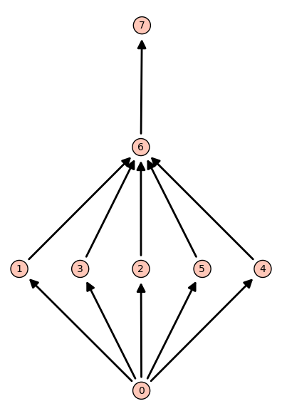
Partial orders on a set of \(8\) elements, up to isomorphism:

sage: C = Posets(8); C
Posets containing 8 elements
sage: C.cardinality()
16999

sage: C.unrank(20).plot()
Graphics object consisting of 20 graphics primitives

One can iterate through all graphs up to isomorphism. For example, there are 34 simple graphs with 5 vertices:

sage: len(list(graphs(5)))
34

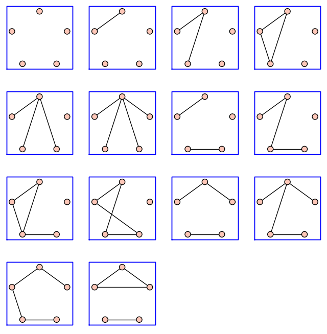
Here are those with at most \(4\) edges:

sage: up_to_four_edges = list(graphs(5, lambda G: G.size() <= 4))
sage: pretty_print(*up_to_four_edges)

However, the set C of these graphs is not yet available in Sage; as a result, the following commands are not yet implemented:

sage: C = Graphs(5)                 # todo: not implemented
sage: C.cardinality()               # todo: not implemented
34
sage: Graphs(19).cardinality()      # todo: not implemented
24637809253125004524383007491432768
sage: Graphs(19).random_element()   # todo: not implemented
Graph on 19 vertices

What we have seen so far also applies, in principle, to finite algebraic structures like the dihedral groups:

sage: G = DihedralGroup(4); G
Dihedral group of order 8 as a permutation group
sage: G.cardinality()
8
sage: G.list()
[(), (1,3)(2,4), (1,4,3,2), (1,2,3,4), (2,4), (1,3), (1,4)(2,3), (1,2)(3,4)]

or the algebra of \(2\times 2\) matrices over the finite field \(\ZZ/2\ZZ\):

sage: C = MatrixSpace(GF(2), 2)
sage: C.list()
[
[0 0]  [1 0]  [0 1]  [0 0]  [0 0]  [1 1]  [1 0]  [1 0]  [0 1]  [0 1]
[0 0], [0 0], [0 0], [1 0], [0 1], [0 0], [1 0], [0 1], [1 0], [0 1],

[0 0]  [1 1]  [1 1]  [1 0]  [0 1]  [1 1]
[1 1], [1 0], [0 1], [1 1], [1 1], [1 1]
]
sage: C.cardinality()
16

Exercise

List all the monomials of degree \(5\) in three variables (see IntegerVectors). Manipulate the ordered set partitions OrderedSetPartitions and standard tableaux (StandardTableaux).

Exercise

List the alternating sign matrices of size \(3\), \(4\), and \(5\) (AlternatingSignMatrices), and try to guess the definition. The discovery and proof of the formula for the enumeration of these matrices (see the method cardinality), motivated by calculations of determinants in physics, is quite a story. In particular, the first proof, given by Zeilberger in 1992 was automatically produced by a computer program. It was 84 pages long, and required nearly a hundred people to verify it.

Exercise

Calculate by hand the number of vectors in \((\ZZ/2\ZZ)^5\), and the number of matrices in \(GL_3(\ZZ/2\ZZ)\) (that is to say, the number of invertible \(3\times 3\) matrices with coefficients in \(\ZZ/2\ZZ\)). Verify your answer with Sage. Generalize to \(GL_n(\ZZ/q\ZZ)\).

Set comprehension and iterators#

We will now show some of the possibilities offered by Python for constructing (and iterating through) sets, with a notation that is flexible and close to usual mathematical usage, and in particular the benefits this yields in combinatorics.

We begin by constructing the finite set \(\{i^2\ \|\ i \in \{1,3,7\}\}\):

sage: [ i^2 for i in [1, 3, 7] ]
[1, 9, 49]

and then the same set, but with \(i\) running from \(1\) to \(9\):

sage: [ i^2 for i in range(1,10) ]
[1, 4, 9, 16, 25, 36, 49, 64, 81]

A construction of this form in Python is called set comprehension. A clause can be added to keep only those elements with \(i\) prime:

sage: [ i^2 for i in range(1,10) if is_prime(i) ]
[4, 9, 25, 49]

Combining more than one set comprehension, it is possible to construct the set \(\{(i,j) \ | \ 1\leq j < i <5\}\):

sage: [ (i,j) for i in range(1,6) for j in range(1,i) ]
[(2, 1), (3, 1), (3, 2), (4, 1), (4, 2), (4, 3),
 (5, 1), (5, 2), (5, 3), (5, 4)]

or to produce Pascal’s triangle:

sage: [[binomial(n,i) for i in range(n+1)] for n in range(10)]
[[1],
 [1, 1],
 [1, 2, 1],
 [1, 3, 3, 1],
 [1, 4, 6, 4, 1],
 [1, 5, 10, 10, 5, 1],
 [1, 6, 15, 20, 15, 6, 1],
 [1, 7, 21, 35, 35, 21, 7, 1],
 [1, 8, 28, 56, 70, 56, 28, 8, 1],
 [1, 9, 36, 84, 126, 126, 84, 36, 9, 1]]

The execution of a set comprehension is accomplished in two steps; first an iterator is constructed, and then a list is filled with the elements successively produced by the iterator. Technically, an iterator is an object with a method next which returns a new value each time it is called, until it is exhausted. For example, the following iterator it:

sage: it = (binomial(3, i) for i in range(4))

returns successively the binomial coefficients \(\binom 3 i\) with \(i=0,1,2,3\):

sage: next(it)
1
sage: next(it)
3
sage: next(it)
3
sage: next(it)
1

When the iterator is finally exhausted, an exception is raised:

sage: next(it)
Traceback (most recent call last):
  ...
StopIteration

More generally, an iterable is a Python object L (a list, a set, …) over whose elements it is possible to iterate. Technically, the iterator is constructed by iter(L). In practice, the commands iter and next are used very rarely, since for loops and list comprehensions provide a much pleasanter syntax:

sage: for s in Subsets(3):
....:     print(s)
{}
{1}
{2}
{3}
{1, 2}
{1, 3}
{2, 3}
{1, 2, 3}

sage: [ s.cardinality() for s in Subsets(3) ]
[0, 1, 1, 1, 2, 2, 2, 3]

What is the point of an iterator? Consider the following example:

sage: sum( [ binomial(8, i) for i in range(9) ] )
256

When it is executed, a list of \(9\) elements is constructed, and then it is passed as an argument to sum to add them up. If, on the other hand, the iterator is passed directly to sum (note the absence of square brackets):

sage: sum( binomial(8, i) for i in range(9) )
256

the function sum receives the iterator directly, and can short-circuit the construction of the intermediate list. If there are a large number of elements, this avoids allocating a large quantity of memory to fill a list which will be immediately destroyed 2.

Most functions that take a list of elements as input will also accept an iterator (or an iterable) instead. To begin with, one can obtain the list (or the tuple) of elements of an iterator as follows:

sage: list(binomial(8, i) for i in range(9))
[1, 8, 28, 56, 70, 56, 28, 8, 1]
sage: tuple(binomial(8, i) for i in range(9))
(1, 8, 28, 56, 70, 56, 28, 8, 1)

We now consider the functions all and any which denote respectively the \(n\)-ary and and or:

sage: all([True, True, True, True])
True
sage: all([True, False, True, True])
False
sage: any([False, False, False, False])
False
sage: any([False, False, True, False])
True

The following example verifies that all primes from \(3\) to \(99\) are odd:

sage: all( is_odd(p) for p in range(3,100) if is_prime(p) )
True

A Mersenne prime is a prime of the form \(2^p -1\). We verify that, for \(p<1000\), if \(2^p-1\) is prime, then \(p\) is also prime:

sage: def mersenne(p): return 2^p -1
sage: [ is_prime(p)
....:   for p in range(1000) if is_prime(mersenne(p)) ]
[True, True, True, True, True, True, True, True, True, True,
 True, True, True, True]

Is the converse true?

Exercise

Try the two following commands and explain the considerable difference in the length of the calculations:

sage: all(   is_prime(mersenne(p))
....:        for p in range(1000) if is_prime(p)  )
False
sage: all( [ is_prime(mersenne(p))
....:        for p in range(1000) if is_prime(p)] )
False

We now try to find the smallest counter-example. In order to do this, we use the Sage function exists:

sage: exists( (p for p in range(1000) if is_prime(p)),
....:         lambda p: not is_prime(mersenne(p)) )
(True, 11)

Alternatively, we could construct an iterator on the counter-examples:

sage: counter_examples = (p for p in range(1000)
....:      if is_prime(p) and not is_prime(mersenne(p)))
sage: next(counter_examples)
11
sage: next(counter_examples)
23

Exercise

What do the following commands do?

sage: cubes = [t**3 for t in range(-999,1000)]
sage: exists([(x,y) for x in cubes for y in cubes],  # long time (3s, 2012)
....:        lambda x_y: x_y[0] + x_y[1] == 218)
(True, (-125, 343))
sage: exists(((x,y) for x in cubes for y in cubes),  # long time (2s, 2012)
....:        lambda x_y: x_y[0] + x_y[1] == 218)
(True, (-125, 343))

Which of the last two is more economical in terms of time? In terms of memory? By how much?

Exercise

Try each of the following commands, and explain its result. If possible, hide the result first and try to guess it before launching the command.

Todo

hide the results by default

Warning

it will be necessary to interrupt the execution of some of the commands

sage: x = var('x')
sage: sum( x^len(s) for s in Subsets(8) )
x^8 + 8*x^7 + 28*x^6 + 56*x^5 + 70*x^4 + 56*x^3 + 28*x^2 + 8*x + 1

sage: sum( x^p.length() for p in Permutations(3) )
x^3 + 2*x^2 + 2*x + 1

sage: factor(sum( x^p.length() for p in Permutations(3) ))
(x^2 + x + 1)*(x + 1)

sage: P = Permutations(5)
sage: all( p in P for p in P )
True

sage: for p in GL(2, 2): print(p); print("")
[1 0]
[0 1]

[0 1]
[1 0]

[0 1]
[1 1]

[1 1]
[0 1]

[1 1]
[1 0]

[1 0]
[1 1]

sage: for p in Partitions(3): print(p)   # not tested
[3]
[2, 1]
[1, 1, 1]
...

sage: for p in Partitions(): print(p)    # not tested
[]
[1]
[2]
[1, 1]
[3]
...

sage: for p in Primes(): print(p)        # not tested
2
3
5
7
...

sage: exists( Primes(), lambda p: not is_prime(mersenne(p)) )
(True, 11)

sage: counter_examples = (p for p in Primes()
....:                    if not is_prime(mersenne(p)))
sage: for p in counter_examples: print(p)   # not tested
11
23
29
37
41
43
47
...

Operations on iterators#

Python provides numerous tools for manipulating iterators; most of them are in the itertools library, which can be imported by:

sage: import itertools

We will demonstrate some applications, taking as a starting point the permutations of \(3\):

sage: list(Permutations(3))
[[1, 2, 3], [1, 3, 2], [2, 1, 3],
 [2, 3, 1], [3, 1, 2], [3, 2, 1]]

We can list the elements of a set by numbering them:

sage: list(enumerate(Permutations(3)))
[(0, [1, 2, 3]), (1, [1, 3, 2]), (2, [2, 1, 3]),
 (3, [2, 3, 1]), (4, [3, 1, 2]), (5, [3, 2, 1])]

or select only the elements in positions 2, 3, and 4 (analogue of l[1:4]):

sage: import itertools
sage: list(itertools.islice(Permutations(3), int(1), int(4)))
[[1, 3, 2], [2, 1, 3], [2, 3, 1]]

To apply a function to all the elements, one can do:

sage: [z.cycle_type() for z in Permutations(3)]
[[1, 1, 1], [2, 1], [2, 1], [3], [3], [2, 1]]

and similarly to select the elements satisfying a certain condition:

sage: [z for z in Permutations(3) if z.has_pattern([1,2])]
[[1, 2, 3], [1, 3, 2], [2, 1, 3], [2, 3, 1], [3, 1, 2]]

Implementation of new iterators#

It is easy to construct new iterators, using the keyword yield instead of return in a function:

sage: def f(n):
....:     for i in range(n):
....:         yield i

After the yield, execution is not halted, but only suspended, ready to be continued from the same point. The result of the function is therefore an iterator over the successive values returned by yield:

sage: g = f(4)
sage: next(g)
0
sage: next(g)
1
sage: next(g)
2
sage: next(g)
3

sage: next(g)
Traceback (most recent call last):
  ...
StopIteration

The function could be used as follows:

sage: [ x for x in f(5) ]
[0, 1, 2, 3, 4]

This model of computation, called continuation, is very useful in combinatorics, especially when combined with recursion. Here is how to generate all words of a given length on a given alphabet:

sage: def words(alphabet,l):
....:    if l == 0:
....:        yield []
....:    else:
....:        for word in words(alphabet, l-1):
....:            for l in alphabet:
....:                yield word + [l]
sage: [ w for w in words(['a','b'], 3) ]
[['a', 'a', 'a'], ['a', 'a', 'b'], ['a', 'b', 'a'],
 ['a', 'b', 'b'], ['b', 'a', 'a'], ['b', 'a', 'b'],
 ['b', 'b', 'a'], ['b', 'b', 'b']]

These words can then be counted by:

sage: sum(1 for w in words(['a','b','c','d'], 10))
1048576

Counting the words one by one is clearly not an efficient method in this case, since the formula \(n^\ell\) is also available; note, though, that this is not the stupidest possible approach - it does, at least, avoid constructing the entire list in memory.

We now consider Dyck words, which are well-parenthesized words in the letters “\((\)” and “\()\)”. The function below generates all the Dyck words of a given length (where the length is the number of pairs of parentheses), using the recursive definition which says that a Dyck word is either empty or of the form \((w_1)w_2\) where \(w_1\) and \(w_2\) are Dyck words:

sage: def dyck_words(l):
....:     if l==0:
....:         yield ''
....:     else:
....:         for k in range(l):
....:             for w1 in dyck_words(k):
....:                 for w2 in dyck_words(l-k-1):
....:                     yield '('+w1+')'+w2

Here are all the Dyck words of length \(4\):

sage: list(dyck_words(4))
['()()()()', '()()(())', '()(())()', '()(()())', '()((()))',
 '(())()()', '(())(())', '(()())()', '((()))()', '(()()())',
 '(()(()))', '((())())', '((()()))', '(((())))']

Counting them, we recover a well-known sequence:

sage: [ sum(1 for w in dyck_words(l)) for l in range(10) ]
[1, 1, 2, 5, 14, 42, 132, 429, 1430, 4862]

Exercise: complete binary tree iterator

Construct an iterator on the set \(C_n\) of complete binary trees with \(n\) leaves (see Enumeration of trees using generating functions).

Hint: Sage 4.8.2 does not yet have a native data structure to represent complete binary trees. One simple way to represent them is to define a formal variable Leaf for the leaves and a formal 2-ary function Node:

sage: var('Leaf')
Leaf
sage: function('Node', nargs=2)
Node

The second tree in Figure: The five complete binary trees with four leaves can be represented by the expression:

sage: tr = Node(Node(Leaf, Node(Leaf, Leaf)), Leaf)

Constructions#

We will now see how to construct new sets starting from these building blocks. In fact, we have already begun to do this with the construction of \(\mathcal P(\mathcal P(\mathcal P(\{1,2,3,4\})))\) in the previous section, and to construct the example of sets of cards in Initial examples.

Consider a large Cartesian product:

sage: C = cartesian_product([Compositions(8), Permutations(20)]); C
The Cartesian product of (Compositions of 8, Standard permutations of 20)
sage: C.cardinality()
311411457046609920000

Clearly, it is impractical to construct the list of all the elements of this Cartesian product! And, in the following example, \(H\) is equipped with the usual combinatorial operations and also its structure as a product group:

sage: G = DihedralGroup(4)
sage: H = cartesian_product([G,G])
sage: H in Groups()
True
sage: H.an_element()
((1,3), (1,3))
sage: t = H([G.gen(0), G.gen(0)])
sage: t
((1,2,3,4), (1,2,3,4))
sage: t*t
((1,3)(2,4), (1,3)(2,4))

We now construct the union of two existing disjoint sets:

sage: C = DisjointUnionEnumeratedSets(
....:       [ Compositions(4), Permutations(3)] )
sage: C
Disjoint union of Family (Compositions of 4,
Standard permutations of 3)
sage: C.cardinality()
14
sage: C.list()
[[1, 1, 1, 1], [1, 1, 2], [1, 2, 1], [1, 3], [2, 1, 1], [2, 2],
[3, 1], [4], [1, 2, 3], [1, 3, 2], [2, 1, 3], [2, 3, 1],
[3, 1, 2], [3, 2, 1]]

It is also possible to take the union of more than two disjoint sets, or even an infinite number of them. We will now construct the set of all permutations, viewed as the union of the sets \(P_n\) of permutations of size \(n\). We begin by constructing the infinite family \(F=(P_n)_{n\in N}\):

sage: F = Family(NonNegativeIntegers(), Permutations); F
Lazy family (<class 'sage.combinat.permutation.Permutations'>(i))_{i in Non negative integers}
sage: F.keys()
Non negative integers
sage: F[1000]
Standard permutations of 1000

Now we can construct the disjoint union \(\bigcup_{n\in \NN}P_n\):

sage: U = DisjointUnionEnumeratedSets(F); U
Disjoint union of
Lazy family (<class 'sage.combinat.permutation.Permutations'>(i))_{i in Non negative integers}

It is an infinite set:

sage: U.cardinality()
+Infinity

which doesn’t prohibit iteration through its elements, though it will be necessary to interrupt it at some point:

sage: for p in U:                # not tested
....:     print(p)
[]
[1]
[1, 2]
[2, 1]
[1, 2, 3]
[1, 3, 2]
[2, 1, 3]
[2, 3, 1]
[3, 1, 2]
...

Note: the above set could also have been constructed directly with:

sage: U = Permutations(); U
Standard permutations

Summary#

Sage provides a library of common enumerated sets, which can be combined by standard constructions, giving a toolbox that is flexible (but which could still be expanded). It is also possible to add new building blocks to Sage with a few lines (see the code in FiniteEnumeratedSets().example()). This is made possible by the uniformity of the interfaces and the fact that Sage is based on an object-oriented language. Also, very large or even infinite sets can be manipulated thanks to lazy evaluation strategies (iterators, etc.).

There is no magic to any of this: under the hood, Sage applies the usual rules (for example, that the cardinality of \(E\times E\) is \(|E|^2\)); the added value comes from the capacity to manipulate complicated constructions. The situation is comparable to Sage’s implementation of differential calculus: Sage applies the usual rules for differentiation of functions and their compositions, where the added value comes from the possibility of manipulating complicated formulas. In this sense, Sage implements a calculus of finite enumerated sets.

Generic algorithms#

Lexicographic generation of lists of integers#

Among the classic enumerated sets, especially in algebraic combinatorics, a certain number are composed of lists of integers of fixed sum, such as partitions, compositions, or integer vectors. These examples can also have supplementary constraints added to them. Here are some examples. We start with the integer vectors with sum \(10\) and length \(3\), with parts bounded below by \(2\), \(4\) and \(2\) respectively:

sage: IntegerVectors(10, 3, min_part=2, max_part=5,
....:                inner=[2, 4, 2]).list()
[[4, 4, 2], [3, 5, 2], [3, 4, 3], [2, 5, 3], [2, 4, 4]]

The compositions of \(5\) with each part at most \(3\), and with length \(2\) or \(3\):

sage: Compositions(5, max_part=3,
....:              min_length=2, max_length=3).list()
[[3, 2], [3, 1, 1], [2, 3], [2, 2, 1], [2, 1, 2], [1, 3, 1],
 [1, 2, 2], [1, 1, 3]]

The strictly decreasing partitions of \(5\):

sage: Partitions(5, max_slope=-1).list()
[[5], [4, 1], [3, 2]]

These sets share the same underlying algorithmic structure, implemented in the more general (and slightly more cumbersome) class IntegerListsLex. This class models sets of vectors \((\ell_0,\dots,\ell_k)\) of non-negative integers, with constraints on the sum and the length, and bounds on the parts and on the consecutive differences between the parts. Here are some more examples:

sage: IntegerListsLex(10, length=3,
....:                 min_part=2, max_part=5,
....:                 floor=[2, 4, 2]).list()
[[4, 4, 2], [3, 5, 2], [3, 4, 3], [2, 5, 3], [2, 4, 4]]

sage: IntegerListsLex(5, min_part=1, max_part=3,
....:                 min_length=2, max_length=3).list()
[[3, 2], [3, 1, 1], [2, 3], [2, 2, 1], [2, 1, 2],
 [1, 3, 1], [1, 2, 2], [1, 1, 3]]

sage: IntegerListsLex(5, min_part=1, max_slope=-1).list()
[[5], [4, 1], [3, 2]]

sage: list(Compositions(5, max_length=2))
[[5], [4, 1], [3, 2], [2, 3], [1, 4]]

sage: list(IntegerListsLex(5, max_length=2, min_part=1))
[[5], [4, 1], [3, 2], [2, 3], [1, 4]]

The point of the model of IntegerListsLex is in the compromise between generality and efficiency. The main algorithm permits iteration through the elements of such a set \(S\) in reverse lexicographic order with a good complexity in most practical use cases. Roughly speaking, the time needed to iterate through all the elements of \(S\) is proportional to the number of elements, where the proportion factor is controlled by the length \(l\) of the longest element of \(S\). In addition, the memory usage is also controlled by \(l\), which is to say negligible in practice.

This algorithm is based on a very general principle for traversing a decision tree, called branch and bound: at the top level, we run through all the possible choices for \(\ell_0\); for each of these choices, we run through all the possible choices for \(\ell_1\), and so on. Mathematically speaking, we have put the structure of a prefix tree on the elements of \(S\): a node of the tree at depth \(k\) corresponds to a prefix \(\ell_0,\dots,\ell_k\) of one (or more) elements of \(S\) (see Figure: The prefix tree of the partitions of 5.).

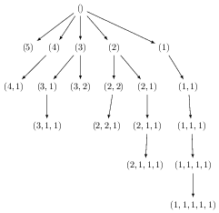
../../_images/prefix-tree-partitions-5.png — Figure: The prefix tree of the partitions of 5.#

The usual problem with this type of approach is to avoid bad decisions which lead to leaving the prefix tree and exploring dead branches; this is particularly problematic because the growth of the number of elements is usually exponential in the depth. It turns out that the constraints listed above are simple enough to be able to reasonably predict when a sequence \(\ell_0,\dots,\ell_k\) is a prefix of some element \(S\). Hence, most dead branches can be pruned.

Integer points in polytopes#

Although the algorithm for iteration in IntegerListsLex is efficient, its counting algorithm is naive: it just iterates over all the elements.

There is an alternative approach to treating this problem: modelling the desired lists of integers as the set of integer points of a polytope, that is to say, the set of solutions with integer coordinates of a system of linear inequalities. This is a very general context in which there exist advanced counting algorithms (e.g. Barvinok), which are implemented in libraries like LattE. Iteration does not pose a hard problem in principle. However, there are two limitations that justify the existence of IntegerListsLex. The first is theoretical: lattice points in a polytope only allow modelling of problems of a fixed dimension (length). The second is practical: at the moment only the library PALP has a Sage interface, and though it offers multiple capabilities for the study of polytopes, in the present application it only produces a list of lattice points, without providing either an iterator or non-naive counting:

sage: A = random_matrix(ZZ, 6, 3, x=7)
sage: L = LatticePolytope(A.rows())
sage: L.points()                               # random
M(4, 1, 0),
M(0, 3, 5),
M(2, 2, 3),
M(6, 1, 3),
M(1, 3, 6),
M(6, 2, 3),
M(3, 2, 4),
M(3, 2, 3),
M(4, 2, 4),
M(4, 2, 3),
M(5, 2, 3)
in 3-d lattice M
sage: L.npoints()                                 # random
11

This polytope can be visualized in 3D with L.plot3d() (see Figure: The polytope L and its integer points, in cross-eyed stereographic perspective.).

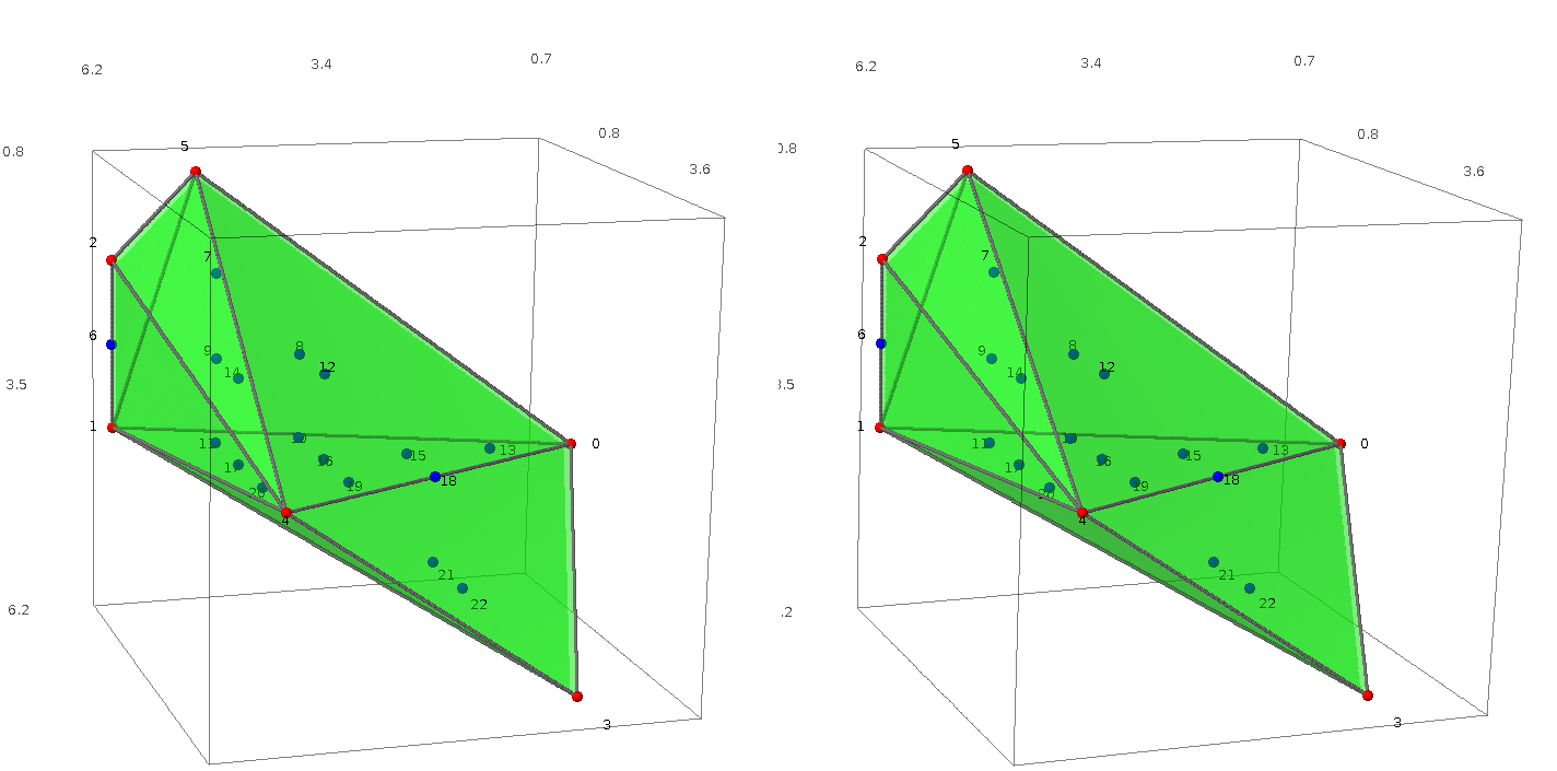
../../_images/polytope.png — Figure: The polytope \(L\) and its integer points, in cross-eyed stereographic perspective.#

Species, decomposable combinatorial classes#

In Enumeration of trees using generating functions, we showed how to use the recursive definition of binary trees to count them efficiently using generating functions. The techniques we used there are very general, and apply whenever the sets involved can be defined recursively (depending on who you ask, such a set is called a decomposable combinatorial class or, roughly speaking, a combinatorial species). This includes all the types of trees, but also permutations, compositions, functional graphs, etc.

Here, we illustrate just a few examples using the Sage library on combinatorial species:

sage: from sage.combinat.species.library import *
sage: o = var('o')

We begin by redefining the complete binary trees; to do so, we stipulate the recurrence relation directly on the sets:

sage: BT = CombinatorialSpecies(min=1)
sage: Leaf =  SingletonSpecies()
sage: BT.define( Leaf + (BT*BT) )

Now we can construct the set of trees with five nodes, list them, count them…:

sage: BT5 = BT.isotypes([o]*5)
sage: BT5.cardinality()
14
sage: BT5.list()
[o*(o*(o*(o*o))), o*(o*((o*o)*o)), o*((o*o)*(o*o)),
 o*((o*(o*o))*o), o*(((o*o)*o)*o), (o*o)*(o*(o*o)),
 (o*o)*((o*o)*o), (o*(o*o))*(o*o), ((o*o)*o)*(o*o),
 (o*(o*(o*o)))*o, (o*((o*o)*o))*o, ((o*o)*(o*o))*o,
 ((o*(o*o))*o)*o, (((o*o)*o)*o)*o]

The trees are constructed using a generic recursive structure; the display is therefore not wonderful. To do better, it would be necessary to provide Sage with a more specialized data structure with the desired display capabilities.

We recover the generating function for the Catalan numbers:

sage: g = BT.isotype_generating_series(); g
z + z^2 + 2*z^3 + 5*z^4 + 14*z^5 + 42*z^6 + 132*z^7 + O(z^8)

which is returned in the form of a lazy power series:

sage: g[100]
227508830794229349661819540395688853956041682601541047340

We finish with the Fibonacci words, which are binary words without two consecutive “\(1\)”s. They admit a natural recursive definition:

sage: Eps =  EmptySetSpecies()
sage: Z0  =  SingletonSpecies()
sage: Z1  =  Eps*SingletonSpecies()
sage: FW  = CombinatorialSpecies()
sage: FW.define(Eps + Z0*FW  +  Z1*Eps + Z1*Z0*FW)

The Fibonacci sequence is easily recognized here, hence the name:

sage: L = FW.isotype_generating_series()[:15]; L
[1, 2, 3, 5, 8, 13, 21, 34, 55, 89, 144, 233, 377, 610, 987]

sage: oeis(L)                                       # optional -- internet
A000045: Fibonacci numbers: F(n) = F(n-1) + F(n-2) with F(0) = 0 and F(1) = 1.
...
...

This is an immediate consequence of the recurrence relation. One can also generate immediately all the Fibonacci words of a given length, with the same limitations resulting from the generic display.

sage: FW3 = FW.isotypes([o]*3)
sage: FW3.list()
[o*(o*(o*{})), o*(o*(({}*o)*{})), o*((({}*o)*o)*{}),
 (({}*o)*o)*(o*{}), (({}*o)*o)*(({}*o)*{})]

Graphs up to isomorphism#

We saw in Some other finite enumerated sets that Sage could generate graphs and partial orders up to isomorphism. We will now describe the underlying algorithm, which is the same in both cases, and covers a substantially wider class of problems.

We begin by recalling some notions. A graph \(G=(V,E)\) is a set \(V\) of vertices and a set \(E\) of edges connecting these vertices; an edge is described by a pair \(\{u,v\}\) of distinct vertices of \(V\). Such a graph is called labelled; its vertices are typically numbered by considering \(V=\{1,2,3,4,5\}\).

In many problems, the labels on the vertices play no role. Typically a chemist wants to study all the possible molecules with a given composition, for example the alkanes with \(n=8\) atoms of carbon and \(2n+2=18\) atoms of hydrogen. He therefore wants to find all the graphs consisting of \(8\) vertices with \(4\) neighbours, and \(18\) vertices with a single neighbour. The different carbon atoms, however, are all considered to be identical, and the same for the hydrogen atoms. The problem of our chemist is not imaginary; this type of application is actually at the origin of an important part of the research in graph theory on isomorphism problems.

Working by hand on a small graph it is possible, as in the example of Some other finite enumerated sets, to make a drawing, erase the labels, and “forget” the geometrical information about the location of the vertices in the plane. However, to represent a graph in a computer program, it is necessary to introduce labels on the vertices so as to be able to describe how the edges connect them together. To compensate for the extra information which we have introduced, we then say that two labelled graphs \(g_1\) and \(g_2\) are isomorphic if there is a bijection from the vertices of \(g_1\) to those of \(g_2\), which maps bijectively the edges of \(g_1\) to those of \(g_2\); an unlabelled graph is then an equivalence class of labelled graphs.

In general, testing if two labelled graphs are isomorphic is expensive. However, the number of graphs, even unlabelled, grows very rapidly. Nonetheless, it is possible to list unlabelled graphs very efficiently considering their number. For example, the program Nauty can list the \(12005168\) simple graphs with \(10\) vertices in \(20\) seconds.

As in Lexicographic generation of lists of integers, the general principle of the algorithm is to organize the objects to be enumerated into a tree that one traverses.

For this, in each equivalence class of labelled graphs (that is to say, for each unlabelled graph) one fixes a convenient canonical representative. The following are the fundamental operations:

Testing whether a labelled graph is canonical
Calculating the canonical representative of a labelled graph

These unavoidable operations remain expensive; one therefore tries to minimize the number of calls to them.

The canonical representatives are chosen in such a way that, for each canonical labelled graph \(G\), there is a canonical choice of an edge whose removal produces a canonical graph again, which is called the father of \(G\). This property implies that it is possible to organize the set of canonical representatives as a tree: at the root, the graph with no edges; below it, its unique child, the graph with one edge; then the graphs with two edges, and so on. The set of children of a graph \(G\) can be constructed by augmentation, adding an edge in all the possible ways to \(G\), and then selecting, from among those graphs, the ones that are still canonical 3. Recursively, one obtains all the canonical graphs.

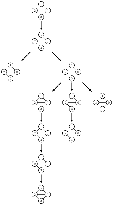
../../_images/prefix-tree-graphs-4.png — Figure: The generation tree of simple graphs with \(4\) vertices.#

In what sense is this algorithm generic? Consider for example planar graphs (graphs which can be drawn in the plane without edges crossing): by removing an edge from a planar graph, one obtains another planar graph; so planar graphs form a subtree of the previous tree. To generate them, exactly the same algorithm can be used, selecting only the children which are planar:

sage: [len(list(graphs(n, property = lambda G: G.is_planar())))
....:  for n in range(7)]
[1, 1, 2, 4, 11, 33, 142]

In a similar fashion, one can generate any family of graphs closed under deletion of an edge, and in particular any family characterized by a forbidden subgraph. This includes for example forests (graphs without cycles), bipartite graphs (graphs without odd cycles), etc. This can be applied to generate:

partial orders, via the bijection with Hasse diagrams which are oriented graphs without cycles and without edges implied by the transitivity of the order relation;
lattices (not implemented in Sage), via the bijection with the meet semi-lattice obtained by deleting the maximal vertex; in this case an augmentation by vertices rather than by edges is used.

REFERENCES:

CMS2012

Alexandre Casamayou, Nathann Cohen, Guillaume Connan, Thierry Dumont, Laurent Fousse, François Maltey, Matthias Meulien, Marc Mezzarobba, Clément Pernet, Nicolas M. Thiéry, Paul Zimmermann Calcul Mathématique avec Sage https://www.sagemath.org/sagebook/french.html

1: Or at least that should be the case; there are still many corners to clean up.
2: Technical detail: range returns an iterator on \(\{0,\dots,8\}\) while range returns the corresponding list. Starting in Python 3.0, range will behave like range, and range will no longer be needed.
3: In practice, an efficient implementation would exploit the symmetries of \(G\), i.e., its automorphism group, to reduce the number of children to explore, and to reduce the cost of each test of canonicity.